Convolutional Neural Network for Product Quality Inspection

20th February 2024

Preface

Neural Network

Deep learning is an exciting invention that has risen in popularity in recent years, but it's beginnings traced back to the 1950s when the earliest prototypes of artificial neural network algorithms were created. The algorithm is named so because it is inspired from our understanding at that time of how our biological brain responds to stimuli from sensory inputs. That is not to say that neural networks are valid representations of how our biological brain works - quite far from that! In fact, the over-sensationalization of neural network is in my opinion doing more harm to actual science than good.

The Architecture of Neural Network

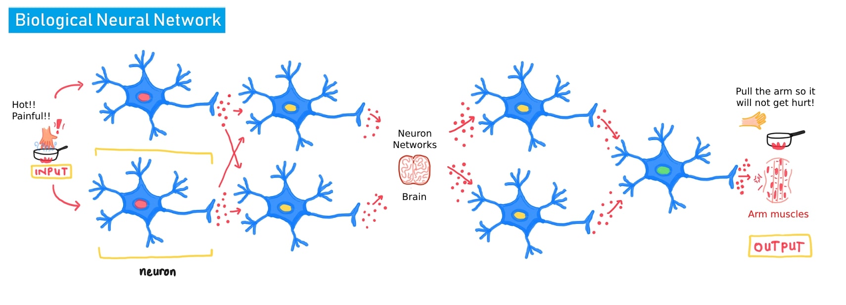
Human nerve system consist of nerve cell named Neuron and each of it combine to creates Networks. Each stimulus/ input from the outside of the body will be accepted by body senses as a signal then it will distributed from one nerve cell to another. The nerve system are spreaded from the tip of the fingers to the brain and continue to all over the body parts.

The nerve system continue to distribute the information from a stimulus/ input, processed in the brain and will be expressed as a body reaction/ activity as a given output or response.

Human Neuron	Artificial Neural Network's Neuron

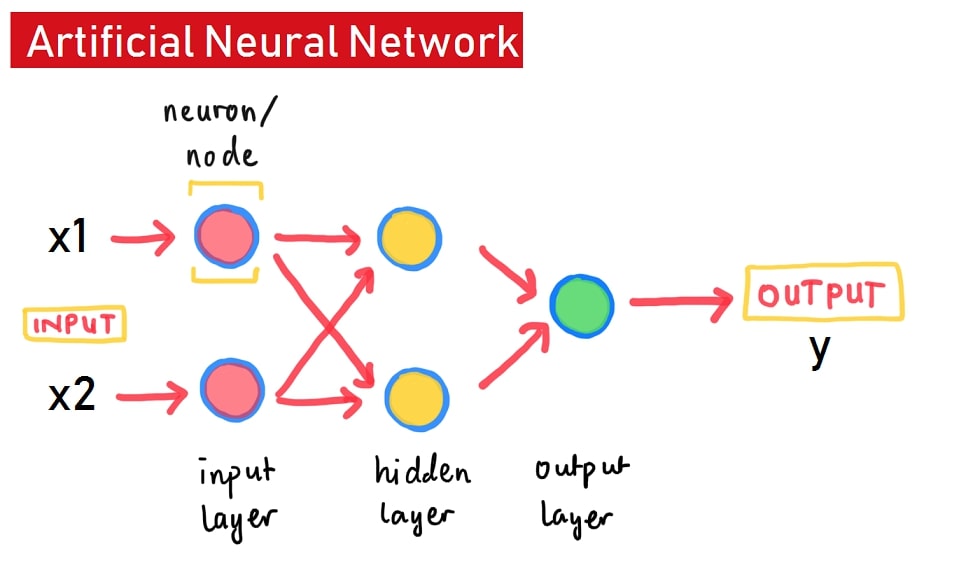
This is the inspiration of the creation of Neural Network Model.

This article is the further usage of Neural Network. For the basic knowledge of Neural Network, kindly please visit this link : Introduction of Neural Network

Background

Casting is a manufacturing process in which liquid material is poured into a mold to solidify. Many types of defects or unwanted irregularities can occur during this process. The industry has its quality inspection department to remove defective products from the production line, but this is very time consuming since it is carried out manually. Furthermore, there is a chance of misclassifying due to human error, causing rejection of the whole product order.

From these problems we will use image data to create a machine learning model. One of the most popular and good methods for working with image datasets is the Convolutional Neural Network (CNN).

This material aims to provide an understanding of the automation of the inspection process by training top-view images of a casted submersible pump impeller using Convolutional Neural Network (CNN).

Convolutional Neural Network

Convolutional Neural Network are nowadays standard architecture to deal with image data. Its history started in 1989 when Yan Lecunn created its first Optical Character Recognition (OCR) model to classify numbers and characters. Due to the flaw of deep neural network activation functions, most of the network will fails of either vanishing gradient or exploding gradient. The problem occurs until in 2011, Yoshua Bengio created Rectified Linear Unit that enables most of deep learning architecture to avoid the problems.

A year after, Alex Krizhevsky re-created Yann Lecunn's CNN and implmented Relu in it. The model was submitted on 2012 Imagenet Competition and the performance was way better than any Deep Neural Network architecture at that time. The model then become the first heavily known CNN that works and its named upon its author, "Alex Net". It marked as the starting point of Deep Learning hype for computer vision.

Convolution Concepts

The concept of convolution is extract those relevant values only and remove all the irrelevant pixels to avoid any unnecessary huge feature to train. This way, our network will have so much lighter feature but with relatively same (or even better) information.

Please take a look at convolutional neural network architecture below :

We just take the relevant values of the car (the blue color) and remove all the irrelevant pixels(the white area).

The end of the network was basically a neural network. Nowadays, these layers are called dense (since all the node are densely connected). Based on the illustration, the convolution part was used to extract important feature from the data before being fed into a dense layers. The convoluted data might be smaller in size but richer in information, resulting in more effective works for the dense layers.

There are two main activity in the convolution, firstly the convolution itself, and the second is pooling.

1. Convolution

To briefly understand how the convolution works, please take alook at below picture of animal then make a guess what kind of animal it is.

Have you make your guess? You probably went for cat, rat, or even a bear. Whatever you have guessed, the interesting part is the process of guessing. There should be some physical characteristic from the image that snaps your brain to think like "Oh, this particular part of the body looks like cat", and that's just how our brain works. It remember particular parts of an object. In fact, it really goods at finding pattern and visual characteristics. If we are given something we don't know, our brain will certainly think of something similar in the past. This is something that we are going to try to mimic using convolution process.

A convolution will extract meaningful information from the data using filters. These filters works just like any filter in real world, it has specific usage and has sensitivity over a very specific means. For eaxmple, think of a UV filter for camera lens. It will block UV lights to reduce the excesssive blue color from the sky. The more UV light on the field, the more this filter will active to tell you that there are UV lights.

Mathematically, the feedforward process of convolutional neural network is called "cross correlation". The term convolution comes from its derivative function when the network do backpropagation. Below are the illustration and mathematical formula on how the network do feedforwards

$$ F \circ I (x,y) = \sum_{j=-N}^{N} \sum_{i=-N}^{N} F(i,j) \times I(x+i, y+j)$$

2. Pooling

If we have convoluted feature extracted from the convolutions process, it may somehow still consists redundant or slightly insignifficant features. Not to mention that the size might explode. The idea of pooling is to summarize and simplify the convolved feature by doing aggreagation over the convolved feature. Remember that we wanted the dense layer to be fed with small yet meaningful features. Below are example of Max Pooling where the convolved feature being summarized into a 2x2 data.

Data Augmentation

Convolutional neural network works well on image data. However, the performance still relies on the quality of the data. In some cases, we don't have enough data to start with. Forcing the model to train on small dataset will heavily increase the probability of being overfit.

To reduce the impact of overfitting, we will do some augmentation to increase the variety of the data and reduce overfitting. Image data works well with augmentation since it won't change the information that much,

There are various way to augment an image, but below are the most common ones:

• Horizontal and Vertical Flip
• Zoom: Zoom in the image
• Shear: Shear image
• Width and Height Shift : Shift the image vertically or horizontally
• Rotation : Rotate the image on specific angle

All those augmentation method are available under keras.preprocessing.image.ImageDataGenerator Class. Not only that, the ImageDataGenerator also provides a few functions to preprocess our data like rescaling or even custom preprocessing function.

Main Course

Now this is the fun part, we will start to create a CNN model to work!

Import Libraries

Before we begin any analysis and modeling, let's import several necessary libraries to work with the data.

# Data Analysis
import pandas as pd
import numpy as np

# Visualization
import matplotlib.pyplot as plt
import seaborn as sns
sns.set()

# Neural Network Model
from keras.preprocessing.image import ImageDataGenerator
from keras.models import Sequential, load_model
from keras.layers import *
from keras.callbacks import ModelCheckpoint

# Evaluation
from sklearn.metrics import confusion_matrix, classification_report

Load the Images

Here is the structure of the folder containing image data:

casting_data
├───test
│   ├───def_front
│   └───ok_front
└───train
    ├───def_front
    └───ok_front

The folder casting_data consists of two subfolders test and train in which each of them has another subfolder: def_front and ok_front denoting the class of our target variable. The images inside train will be used for model fitting and validation, while test will be used purely for testing the model performance on unseen images.

#Data Augmentation

train_generator = ImageDataGenerator(rotation_range = 360,
                                     width_shift_range = 0.05,
                                     height_shift_range = 0.05,
                                     shear_range = 0.05,
                                     zoom_range = 0.05,
                                     horizontal_flip = True,
                                     vertical_flip = True,
                                     brightness_range = [0.75, 1.25],
                                     rescale = 1./255,
                                     validation_split = 0.2)

We define another set of value for the flow_from_directory parameters:

• IMAGE_DIR: The directory where the image data is stored.
• IMAGE_SIZE: The dimension of the image (300 px by 300 px).
• BATCH_SIZE: Number of images that will be loaded and trained at one time.
• SEED_NUMBER: Ensure reproducibility.
• color_mode = "grayscale": Treat our image with only one channel color.
• class_mode and classes define the target class of our problem. In this case, we denote the defect class as positive (1), and ok as a negative class.
• shuffle = True to make sure the model learns the defect and ok images alternately.

IMAGE_DIR = "data_input/casting_data/"
IMAGE_SIZE = (300, 300)
BATCH_SIZE = 64
SEED_NUMBER = 123

gen_args = dict(target_size = IMAGE_SIZE,
                color_mode = "grayscale",
                batch_size = BATCH_SIZE,
                class_mode = "binary",
                classes = {"ok_front": 0, "def_front": 1},
                seed = SEED_NUMBER)

train_dataset = train_generator.flow_from_directory(
                                        directory = IMAGE_DIR + "train",
                                        subset = "training", shuffle = True, **gen_args)
validation_dataset = train_generator.flow_from_directory(
                                        directory = IMAGE_DIR + "train",
                                        subset = "validation", shuffle = True, **gen_args)

Found 5307 images belonging to 2 classes.
Found 1326 images belonging to 2 classes.

We will not perform any data augmentation on the test data.

test_generator = ImageDataGenerator(rescale = 1./255)
test_dataset = test_generator.flow_from_directory(directory = IMAGE_DIR + "test",
                                                  shuffle = False,
                                                  **gen_args)

Found 715 images belonging to 2 classes.

Visualize the Image

We successfully load and apply on-the-fly data augmentation according to the specified parameters. Now, in this section, we visualize the image to make sure that it is loaded correctly.

Visualize Image in Batch

Visualize the first batch (BATCH_SIZE = 64) of the training dataset (images with data augmentation) and also the test dataset (images without data augmentation).

mapping_class = {0: "ok", 1: "defect"}
mapping_class

{0: 'ok', 1: 'defect'}

def visualizeImageBatch(dataset, title):
    images, labels = next(iter(dataset))
    images = images.reshape(BATCH_SIZE, *IMAGE_SIZE)
    fig, axes = plt.subplots(8, 8, figsize=(16,16))

    for ax, img, label in zip(axes.flat, images, labels):
        ax.imshow(img, cmap = "gray")
        ax.axis("off")
        ax.set_title(mapping_class[label], size = 20)

    plt.tight_layout()
    fig.suptitle(title, size = 30, y = 1.05, fontweight = "bold")
    plt.show()
    
    return images

train_images = visualizeImageBatch(train_dataset,
                                   "FIRST BATCH OF THE TRAINING IMAGES\n(WITH DATA AUGMENTATION)")

test_images = visualizeImageBatch(test_dataset,
                                  "FIRST BATCH OF THE TEST IMAGES\n(WITHOUT DATA AUGMENTATION)")

Visualize Detailed Image

Let's also take a look on the detailed image by each pixel. Instead of plotting 300 pixels by 300 pixels (which computationally expensive), we take a small part of 25 pixels by 25 pixels only

img = np.squeeze(train_images[4])[75:100, 75:100]

fig = plt.figure(figsize = (15, 15))
ax = fig.add_subplot(111)
ax.imshow(img, cmap = "gray")
ax.axis("off")

w, h = img.shape
for x in range(w):
    for y in range(h):
        value = img[x][y]
        ax.annotate("{:.2f}".format(value), xy = (y,x),
                    horizontalalignment = "center",
                    verticalalignment = "center",
                    color = "white" if value < 0.4 else "black")

These are the example of values that we are going to feed into our CNN architecture.

Training the Network

As mentioned earlier, we are going to train a CNN model to classify the casting product image. CNN is used as an automatic feature extractor from the images so that it can learn how to distinguish between defect and ok casted products. It effectively uses the adjacent pixel to downsample the image and then use a prediction (fully-connected) layer to solve the classification problem. This is a simple illustration by Udacity on how the layers are arranged sequentially:

Define Architecture

Here is the detailed architecture that we are going to use:

1. First convolutional layer: consists of 32 filters with kernel_size matrix 3 by 3. Using 2-pixel strides at a time, reduce the image size by half.
2. First pooling layer: Using max-pooling matrix 2 by 2 (pool_size) and 2-pixel strides at a time further reduce the image size by half.
3. Second convolutional layer: Just like the first convolutional layer but with 16 filters only.
4. Second pooling layer: Same as the first pooling layer.
5. Flattening: Convert two-dimensional pixel values into one dimension, so that it is ready to be fed into the fully-connected layer.
6. First dense layer + Dropout: consists of 128 units and 1 bias unit. Dropout of rate 20% is used to prevent overfitting.
7. Second dense layer + Dropout: consists of 64 units and 1 bias unit. Dropout of rate 20% is also used to prevent overfitting.
8. Output layer: consists of only one unit and activation is a sigmoid function to convert the scores into a probability of an image being defect.

For every layer except output layer, we use Rectified Linear Unit (ReLU) activation function.

model_cnn = Sequential(
    [
        # First convolutional layer
        Conv2D(filters = 32,
               kernel_size = 3,
               strides = 2,
               activation = "relu",
               input_shape = IMAGE_SIZE + (1, )),
        
        # First pooling layer
        MaxPooling2D(pool_size = 2,
                     strides = 2),
        
        # Second convolutional layer
        Conv2D(filters = 16,
               kernel_size = 3,
               strides = 2,
               activation = "relu"),
        
        # Second pooling layer
        MaxPooling2D(pool_size = 2,
                     strides = 2),
        
        # Flattening
        Flatten(),
        
        # Fully-connected layer
        Dense(128, activation = "relu"),
        Dropout(rate = 0.2),
        
        Dense(64, activation = "relu"),
        Dropout(rate = 0.2),
        
        Dense(1, activation = "sigmoid")
    ]
)

model_cnn.summary()

Model: "sequential"
_________________________________________________________________
 Layer (type)                Output Shape              Param #   
=================================================================
 conv2d (Conv2D)             (None, 149, 149, 32)      320       
                                                                 
 max_pooling2d (MaxPooling2D  (None, 74, 74, 32)       0         
 )                                                               
                                                                 
 conv2d_1 (Conv2D)           (None, 36, 36, 16)        4624      
                                                                 
 max_pooling2d_1 (MaxPooling  (None, 18, 18, 16)       0         
 2D)                                                             
                                                                 
 flatten (Flatten)           (None, 5184)              0         
                                                                 
 dense (Dense)               (None, 128)               663680    
                                                                 
 dropout (Dropout)           (None, 128)               0         
                                                                 
 dense_1 (Dense)             (None, 64)                8256      
                                                                 
 dropout_1 (Dropout)         (None, 64)                0         
                                                                 
 dense_2 (Dense)             (None, 1)                 65        
                                                                 
=================================================================
Total params: 676,945
Trainable params: 676,945
Non-trainable params: 0
_________________________________________________________________

Compile the Model

Next, we specify how the model backpropagates or update the weights after each batch feed-forward. We use adam optimizer and a loss function binary cross-entropy since we are dealing with binary classification problem. The metrics used to monitor the training progress is accuracy.

Imagine how backpropagates, update weights and feed-forward works in a human brain on the process of thinking and doing action:

You want to make a cup of coffee and you starts to boil the water. During this time, you are curious if the water is boiling or not so you keep opening the lid to make sure that there is a bubble coming from the bottom of the kettle, telling you that it is ready.

Turns out on that day and condition, the water is boiling after 10 minutes, but you checked it on the 8th minute, so:

• Backpropagates is the step of processing the information that you received, which realized that on the minute of 8th, the water hasn't boiling yet.

• Update Weights is the step when you learned that you need more than 8 minutes to boil the water and thinking of adding some more time to wait.

• Feed-Forward is the step when, after you Update the Weights, you are now checking the water on the 9th minute.

As you see on the Feed-Forward step, our brain are still wrongly guessing on how long the water will be boiling, so these three steps will keep repeating until you reached the condition that you are quite confident and correctly guessed, which is on the 10th minute.

model_cnn.compile(optimizer = 'adam',
              loss = 'binary_crossentropy',
              metrics = ['accuracy'])

Model Fitting

checkpoint = ModelCheckpoint('model/cnn_casting_inspection_model.hdf5',
                             verbose = 1,
                             save_best_only = True,
                             monitor='val_loss',
                             mode='min')

model_cnn.fit(train_dataset,
                    validation_data = validation_dataset,
                    batch_size = 16,
                    epochs = 15,
                    callbacks = [checkpoint],
                    verbose = 1)

Epoch 1/15
83/83 [==============================] - ETA: 0s - loss: 0.6804 - accuracy: 0.5610
Epoch 00001: val_loss improved from inf to 0.63409, saving model to model\cnn_casting_inspection_model.hdf5
83/83 [==============================] - 148s 2s/step - loss: 0.6804 - accuracy: 0.5610 - val_loss: 0.6341 - val_accuracy: 0.6094
Epoch 2/15
83/83 [==============================] - ETA: 0s - loss: 0.5973 - accuracy: 0.6424
Epoch 00002: val_loss improved from 0.63409 to 0.55821, saving model to model\cnn_casting_inspection_model.hdf5
83/83 [==============================] - 141s 2s/step - loss: 0.5973 - accuracy: 0.6424 - val_loss: 0.5582 - val_accuracy: 0.6923
Epoch 3/15
83/83 [==============================] - ETA: 0s - loss: 0.5542 - accuracy: 0.6800
Epoch 00003: val_loss improved from 0.55821 to 0.50233, saving model to model\cnn_casting_inspection_model.hdf5
83/83 [==============================] - 112s 1s/step - loss: 0.5542 - accuracy: 0.6800 - val_loss: 0.5023 - val_accuracy: 0.7315
Epoch 4/15
83/83 [==============================] - ETA: 0s - loss: 0.5255 - accuracy: 0.6989
Epoch 00004: val_loss improved from 0.50233 to 0.48971, saving model to model\cnn_casting_inspection_model.hdf5
83/83 [==============================] - 89s 1s/step - loss: 0.5255 - accuracy: 0.6989 - val_loss: 0.4897 - val_accuracy: 0.7300
Epoch 5/15
83/83 [==============================] - ETA: 0s - loss: 0.4771 - accuracy: 0.7428
Epoch 00005: val_loss improved from 0.48971 to 0.43967, saving model to model\cnn_casting_inspection_model.hdf5
83/83 [==============================] - 90s 1s/step - loss: 0.4771 - accuracy: 0.7428 - val_loss: 0.4397 - val_accuracy: 0.7655
Epoch 6/15
83/83 [==============================] - ETA: 0s - loss: 0.4493 - accuracy: 0.7588
Epoch 00006: val_loss improved from 0.43967 to 0.38947, saving model to model\cnn_casting_inspection_model.hdf5
83/83 [==============================] - 89s 1s/step - loss: 0.4493 - accuracy: 0.7588 - val_loss: 0.3895 - val_accuracy: 0.8130
Epoch 7/15
83/83 [==============================] - ETA: 0s - loss: 0.3725 - accuracy: 0.8159
Epoch 00007: val_loss improved from 0.38947 to 0.31833, saving model to model\cnn_casting_inspection_model.hdf5
83/83 [==============================] - 84s 1s/step - loss: 0.3725 - accuracy: 0.8159 - val_loss: 0.3183 - val_accuracy: 0.8620
Epoch 8/15
83/83 [==============================] - ETA: 0s - loss: 0.3384 - accuracy: 0.8487
Epoch 00008: val_loss improved from 0.31833 to 0.30089, saving model to model\cnn_casting_inspection_model.hdf5
83/83 [==============================] - 83s 994ms/step - loss: 0.3384 - accuracy: 0.8487 - val_loss: 0.3009 - val_accuracy: 0.8771
Epoch 9/15
83/83 [==============================] - ETA: 0s - loss: 0.2875 - accuracy: 0.8709
Epoch 00009: val_loss improved from 0.30089 to 0.24045, saving model to model\cnn_casting_inspection_model.hdf5
83/83 [==============================] - 83s 1s/step - loss: 0.2875 - accuracy: 0.8709 - val_loss: 0.2404 - val_accuracy: 0.9012
Epoch 10/15
83/83 [==============================] - ETA: 0s - loss: 0.2340 - accuracy: 0.9079
Epoch 00010: val_loss improved from 0.24045 to 0.19629, saving model to model\cnn_casting_inspection_model.hdf5
83/83 [==============================] - 127s 2s/step - loss: 0.2340 - accuracy: 0.9079 - val_loss: 0.1963 - val_accuracy: 0.9178
Epoch 11/15
83/83 [==============================] - ETA: 0s - loss: 0.2441 - accuracy: 0.8943
Epoch 00011: val_loss did not improve from 0.19629
83/83 [==============================] - 114s 1s/step - loss: 0.2441 - accuracy: 0.8943 - val_loss: 0.2079 - val_accuracy: 0.9201
Epoch 12/15
83/83 [==============================] - ETA: 0s - loss: 0.2150 - accuracy: 0.9120
Epoch 00012: val_loss did not improve from 0.19629
83/83 [==============================] - 97s 1s/step - loss: 0.2150 - accuracy: 0.9120 - val_loss: 0.2085 - val_accuracy: 0.9027
Epoch 13/15
83/83 [==============================] - ETA: 0s - loss: 0.1831 - accuracy: 0.9229
Epoch 00013: val_loss improved from 0.19629 to 0.16699, saving model to model\cnn_casting_inspection_model.hdf5
83/83 [==============================] - 104s 1s/step - loss: 0.1831 - accuracy: 0.9229 - val_loss: 0.1670 - val_accuracy: 0.9321
Epoch 14/15
83/83 [==============================] - ETA: 0s - loss: 0.1840 - accuracy: 0.9226
Epoch 00014: val_loss improved from 0.16699 to 0.12696, saving model to model\cnn_casting_inspection_model.hdf5
83/83 [==============================] - 95s 1s/step - loss: 0.1840 - accuracy: 0.9226 - val_loss: 0.1270 - val_accuracy: 0.9548
Epoch 15/15
83/83 [==============================] - ETA: 0s - loss: 0.1497 - accuracy: 0.9412
Epoch 00015: val_loss did not improve from 0.12696
83/83 [==============================] - 82s 983ms/step - loss: 0.1497 - accuracy: 0.9412 - val_loss: 0.1531 - val_accuracy: 0.9351

<keras.callbacks.History at 0x27b544cbd00>

Training Evaluation

Let's plot both loss and accuracy metrics for train and validation data based on each epoch.

plt.subplots(figsize = (8, 6))
sns.lineplot(data = pd.DataFrame(model_cnn.history.history,
                                 index = range(1, 1+len(model_cnn.history.epoch))))
plt.title("TRAINING EVALUATION", fontweight = "bold", fontsize = 20)
plt.xlabel("Epochs")
plt.ylabel("Metrics")

plt.legend(labels = ['val loss', 'val accuracy', 'train loss', 'train accuracy'])
plt.show()

We can conclude that the model is not overfitting the data since both train loss and val loss simultaneously dropped towards zero. Also, both train accuracy and val accuracy increase towards 100%.

Testing on Unseen Images

Our model performs very well on the training and validation dataset which uses augmented images. Now, we test our model performance with unseen and unaugmented images.

best_model = load_model("model/cnn_casting_inspection_model.hdf5")

y_pred_prob = best_model.predict(test_dataset)

The output of the prediction is in the form of probability. We use THRESHOLD = 0.5 to separate the classes. If the probability is greater or equal to the THRESHOLD, then it will be classified as defect, otherwise ok.

THRESHOLD = 0.5
y_pred_class = (y_pred_prob >= THRESHOLD).reshape(-1,)
y_true_class = test_dataset.classes[test_dataset.index_array]

pd.DataFrame(
    confusion_matrix(y_true_class, y_pred_class),
    index = [["Actual", "Actual"], ["ok", "defect"]],
    columns = [["Predicted", "Predicted"], ["ok", "defect"]],
)

		Predicted
		ok	defect
Actual	ok	260	2
	defect	5	448

print(classification_report(y_true_class, y_pred_class, digits = 4))

              precision    recall  f1-score   support

           0     0.9811    0.9924    0.9867       262
           1     0.9956    0.9890    0.9922       453

    accuracy                         0.9902       715
   macro avg     0.9883    0.9907    0.9895       715
weighted avg     0.9903    0.9902    0.9902       715

According to the problem statement, we want to minimize the case of False Negative, where the defect product is misclassified as ok. This can cause the whole order to be rejected and create a big loss for the company. Therefore, in this case, we prioritize Recall over Precision.

But if we take into account the cost of re-casting a product, we have to minimize the case of False Positive also, where the ok product is misclassified as defect. Therefore we can prioritize the F1 score which combines both Recall and Precision.

On test dataset, the model achieves a very good result as follow:

• Accuracy: 98.90%
• Recall: 99.34%
• Precision: 99.56%
• F1 score: 99.22%

---

Conclusion

By using CNN and on-the-fly data augmentation, the performance of our model in training, validation and test images is almost perfect, reaching 98-99% accuracy and F1 score. We can utilize this model by embedding it into a surveillance camera where the system can automatically separate defective product from the production line. This method surely can reduce human error and human resources on manual inspection, but it still needs supervision from human since the model is not 100% correct at all times.

---

External Links:

• Adam
• HDF5 Data Type
• Keras Sequential Model
• Keras Dense Layer
• L1 vs L2 Regularization
• Neuron Transmits Messages In The Brain - Genetic Science Learning Center
• Relu
• RMSProp